Interaction surface: exact fixed-host pull-out (A0)
This benchmark verifies the shaft quadrature, the axial beam transfer, the constant-capacity return mapping and the committed plastic slip of *Embedded region, interaction-surface against a closed-form solution, before host-stress recovery and soil nonlinearity are introduced.
Model
A straight vertical pile (nine u2-beam-3D elements between \(z=10\) m and \(z=5\) m) is embedded in a block of u8-solid-3d elements (720 elements, 2.83 m x 2.83 m in plan with an O-grid around the pile, 10 m high) whose nodes are all fixed, rendering the host rigid. Only the shaft interaction surface is active (no base disk, no ghost zone); the pile head is pulled upwards by a prescribed displacement of \(w=3\) mm and the toe is axially free. The interaction surface uses four coupling points per ring (np=4).
| Quantity | Value |
|---|---|
| Diameter of the interaction surface \(D\) | \(0.20\,\mathrm m\) |
| Embedded length \(L\) | \(5.0\,\mathrm m\) |
| Axial rigidity of the beam \(EA\) | \(9.42478\times10^{5}\,\mathrm{kN}\) (\(A=0.031416\,\mathrm{m^2}\), \(E=3\times10^{7}\,\mathrm{kPa}\)) |
| Tangential stiffness \(k_t\) | \(1.0\times10^{5}\,\mathrm{kN/m^3}\) |
| Normal stiffness \(k_n\) | \(0\) (no normal coupling) |
| Constant shaft capacity \(t_{\mathrm{ult}}\) | \(100\,\mathrm{kPa}\) |
| Base coupling, ghost zone | inactive |
*Embedded region, interaction-surface, type=constant, np=4, ghost=no
embedded-pile-1-shaft, host, none, 0.2, 100000, 0, 0, 100, 0

*Step, name=step 1, inc=1e4, maxiter=32, miniter=1
*Static
0.01, 1, 0.001, 0.1
*Boundary, amplitude=amplitude 1
embedded-pile-1-head, u3, 0.003
*Boundary
host, u1, 0
host, u2, 0
host, u3, 0
Input files
Download the input files (mesh, calculation, material definitions) and the evaluation script here. Run with numgeo inp=embedded-beam-benchmark-A0-calculation out=A0.
The circumference is \(P=\pi D\). With fixed host displacements, the elastic transfer parameter is
The same \(\lambda\), \(Q_y\) and \(Q_{\mathrm{ult}}\) are obtained for any combination of \(D\), \(k_t\) and \(t_{\mathrm{ult}}\) with equal \(Pk_t\) and \(Pt_{\mathrm{ult}}\); the manuscript version of this benchmark uses \(D=1\) m, \(k_t=2\times10^4\) kN/m³ and \(t_{\mathrm{ult}}=20\) kPa.
Closed-form solution
For prescribed head displacement \(w\) and axially free toe, the elastic solution (distance \(x\) from the pile head) is
First yield occurs at the pile head at
If \(a\) denotes the yielded length measured from the pile head and \(u_y=t_{\mathrm{ult}}/k_t\), the partially yielded solution reads
Full yield gives
Results
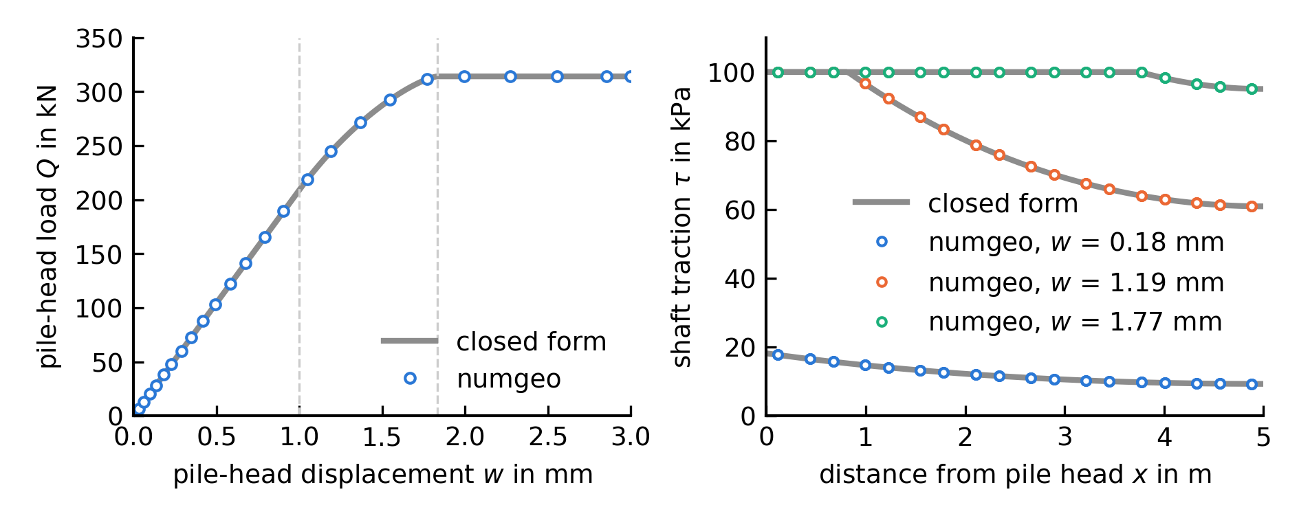
Figure 1: pile-head response (left) and shaft traction distribution at three stages of loading (right) compared with the closed-form solution. The dashed lines mark \(w_y\) and \(w_{\mathrm{full}}\).
The numerical curve coincides with the closed-form solution through the elastic, partially yielded and fully yielded ranges. In the elastic range the pile-head load is 0.12 % above the closed-form value - the discretisation error of nine two-node beam elements with two integration stations each - and the fully mobilised capacity \(Q_{\mathrm{ult}}=314.159\) kN is reproduced exactly (the tributary areas of the 72 coupling points sum to \(\pi DL\)). The shaft tractions read from the diagnostic file embedded-surface-interactions.res follow the analytical distribution, including the yielded zone that propagates from the pile head at \(w=1.19\) mm. Every increment converges in one equilibrium iteration (two in the first increment).
| \(w\) (mm) | \(Q\) numgeo (kN) | \(Q\) closed form (kN) | deviation |
|---|---|---|---|
| 0.492 | 103.10 | 102.98 | 0.12 % |
| 0.904 | 189.36 | 189.14 | 0.12 % |
| 1.191 | 244.66 | 244.51 | 0.06 % |
| 1.548 | 292.88 | 292.64 | 0.08 % |
| 1.995 | 314.16 | 314.16 | 0.00 % |
| 3.000 | 314.16 | 314.16 | 0.00 % |
This verifies:
- the integration of the shaft area \(\pi D L\);
- the equal-and-opposite beam-host force transfer;
- the axial beam stiffness and the sign convention;
- the radial return to the constant shaft capacity;
- the storage and commitment of the plastic shaft slip;
- the algorithmic tangential stiffness (quadratic convergence).
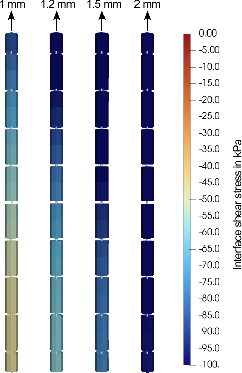
Figure 2: reconstructed shaft surface (VTK output variable embedded) during progressive yielding.
The displayed quadrilaterals are post-processing cells, not interaction finite elements. Every cell represents one coupling-point tributary area. The small axial spaces separate cells centred at adjacent beam integration stations and have no mechanical significance.