Interaction surface: axially loaded pile (A1-A3)
This benchmark group assesses the pressure source for shaft friction, stress recovery, base mobilisation, base-disk quadrature, host-mesh sensitivity, ghost-zone geometry and combined shaft–base response. The comparisons use resolved axisymmetric continuum models of the same pile.
Common model
A vertical pile of diameter \(D=0.80\,\mathrm m\) and embedded length \(L=8.0\,\mathrm m\) is installed wished in place in homogeneous dry sand.
| Quantity | Value |
|---|---|
| Soil Young's modulus \(E_s\) | \(50\,\mathrm{MPa}\) |
| Soil Poisson ratio \(\nu_s\) | \(0.30\) |
| Soil unit weight \(\gamma_s\) | \(20\,\mathrm{kN/m^3}\) |
| Soil cohesion \(c'\) | \(1.0\,\mathrm{kPa}\) |
| Soil friction angle \(\varphi'\) | \(32^\circ\) |
| Soil dilation angle \(\psi'\) | \(0^\circ\) |
| Initial earth-pressure coefficient \(K_0\) | \(0.4701\) |
| Pile Young's modulus \(E_p\) | \(30\,\mathrm{GPa}\) |
| Continuum pile Poisson ratio \(\nu_p\) | \(0.20\) in A1; \(0\) in A2 and A3 |
| Interface reduction \(R_{\mathrm{inter}}\) | \(0.75\) |
| Interface cohesion \(c_i\) | \(0.75\,\mathrm{kPa}\) |
| \(\tan\varphi_i\) | \(0.4686\) |
The zero Poisson ratio in the A2 and A3 continuum pile prevents radial pile expansion from entering the assessment of the base relation; a companion calculation with \(\nu_p=0.20\) is used as a sensitivity check.
The continuum reference (axisymmetric, AX-FE in the figures) extends \(10\,\mathrm m\) radially and \(20\,\mathrm m\) in depth. The embedded models of the mesh study use a \(10\,\mathrm m\) cube with the regular host sequence \(\Delta=1.60\), \(0.80\), \(0.40\) and \(0.20\,\mathrm m\); additional shifted and biased meshes separate element size from mesh position and topology. The input files provided below use a cylindrical host of \(20\,\mathrm m\) diameter and \(20\,\mathrm m\) height (pile head at the ground surface \(z=20\,\mathrm m\), toe at \(z=12\,\mathrm m\)) with u8-solid-3d elements of about \(0.8\,\mathrm m\) (A1, A2: 8100 elements) and \(0.6\,\mathrm m\) with a local vertical refinement around the toe (A3: 19008 elements); the pile consists of 20 u2-beam-3d elements.
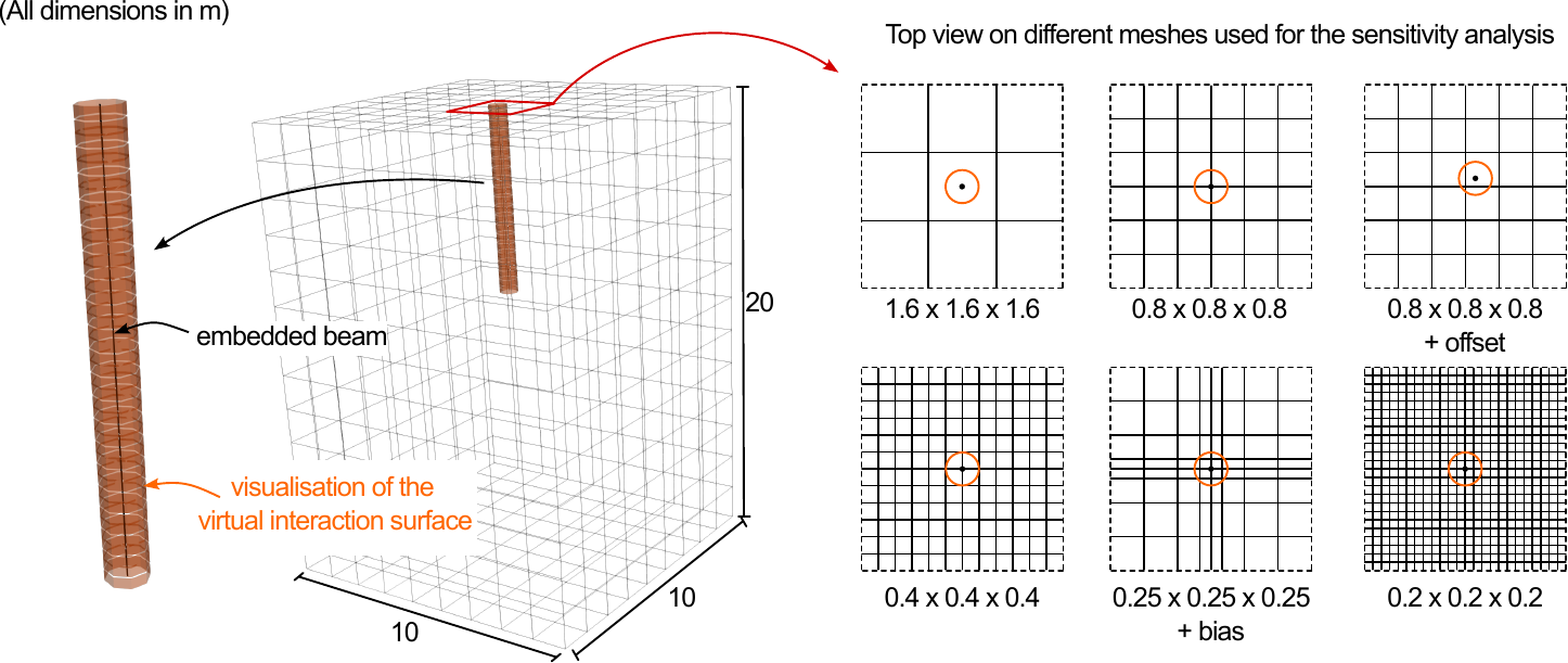
Interaction-surface model and host discretisations used in the axial benchmarks.
A mass-neutral convention is used: the superimposed beam adds no weight to the host material already occupying the virtual pile volume. Pull-out resistance is reported net of the continuum pile weight; compression loads are increments relative to the converged pile-activation state.
Input files
Input files
Download the input files of A1, A2 and A3 (mesh, calculation file and material definitions each). Run with numgeo inp=calculation out=A1 (A1, A2) and numgeo inp=MCSoil-Nlocal-RGauss-B-loc-Hyperbolic2-Ghost-flat-calculation out=A3 (A3).
All three analyses consist of a single *Static step with the geostatic initial stress (\(K_0=0.4701\)) and the self-weight applied instantly; the pile head displacement is prescribed with a ramp amplitude. The pile is present from the beginning with its real stiffness (the initial stresses are in equilibrium with the self-weight, hence no settlement occurs before loading). The embedded-region definitions read
** A1: Mohr-Coulomb shaft, recovered soil stress, no base, no ghost zone, tension
*Embedded region, interaction-surface, type=mohr-coulomb, sigma=soil, recovery=gaussian, ghost=no
embedded-pile-1-shaft, host, none, 0.8, 69358, 762933, 0, 0.75, 25.11, -1

** A2: frictionless shaft, capped hyperbolic base, ghost zone with toe half-sphere, compression
*Embedded region, interaction-surface, type=mohr-coulomb, sigma=soil, recovery=gaussian, ghost=yes, baselaw=hyperbolic, bfac=18.48, bexp=0.2553
embedded-pile-1-shaft, host, embedded-pile-1-toe, 0.8, 43760, 481357, 264413, 1e-06, 0, 1691, 75000, 0.3

** A3: Mohr-Coulomb shaft and capped hyperbolic base, ghost zone without toe half-sphere, compression
*Embedded region, interaction-surface, type=mohr-coulomb, sigma=soil, recovery=gaussian, ghost=shaft, nb=1, baselaw=hyperbolic, bfac=18.48, bexp=0.2553
embedded-pile-1-shaft, host, embedded-pile-1-toe, 0.8, 43760, 481357, 264413, 0.75, 25.11, 1691, 75000, 0.3
The interface stiffnesses follow the estimates of the Theory Manual with \(h=0.8\,\mathrm m\), \(\nu_i=0.45\) and \(\beta=1\) (A2, A3: \(k_t=43.76\), \(k_n=481.4\), \(k_b=264.4\,\mathrm{MN/m^3}\)) or \(\beta=0.5\) (A1: \(k_t=69.4\), \(k_n=762.9\,\mathrm{MN/m^3}\)). In A2 the frictionless shaft is obtained with a Mohr-Coulomb interface of negligible strength (\(c=10^{-6}\) kPa, \(\varphi=0\)). The results obtained with these files are reported at the end of each section ("reproduction"); the figures and tables of the sections themselves are those of the manuscript.
A1: shaft resistance under axial tension
The embedded base is inactive. The pile-head reaction is carried entirely by the frictional shaft.
For interpretation, the geostatic fixed-pressure estimate is
This estimate excludes pressure evolution, pile contraction, opening and end effects; it is not a continuum reference solution.
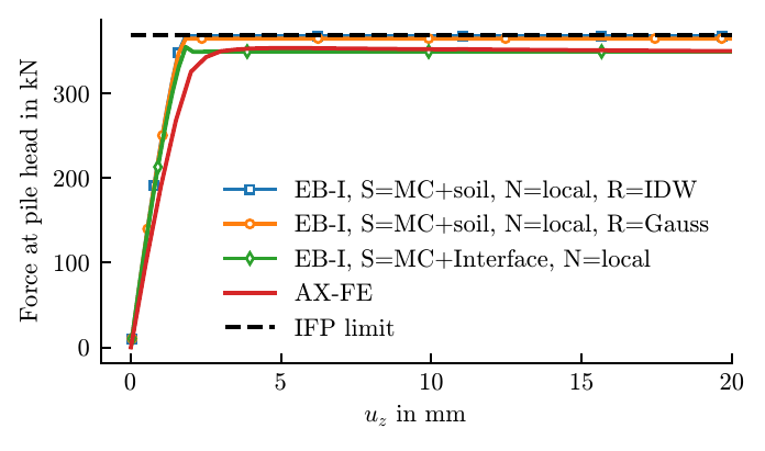
Net pull-out resistance for the pressure-source variants and the axisymmetric reference.
Global comparison
| Model | Stiffness multiplier | Terminal resistance \(Q_{20}\) (kN) | \(u_{95}\) (mm) |
|---|---|---|---|
| Axisymmetric continuum | -- | 350.3 | 2.20 |
| Soil stress, inverse-distance recovery | 1 | 368.0 | 1.60 |
| Soil stress, Gaussian recovery | 0.1 | 363.7 | 5.19 |
| Soil stress, Gaussian recovery | 1 | 365.2 | 1.58 |
| Soil stress, Gaussian recovery | 10 | 366.4 | 1.27 |
| Interface pressure | 0.1 | 369.1 | 5.33 |
| Interface pressure | 1 | 349.8 | 1.60 |
| Interface pressure | 10 | 330.8 | 1.18 |
For the soil-stress source, changing the common tangential and normal stiffness multiplier by two orders of magnitude alters terminal resistance by less than \(0.8\%\), while mobilisation becomes faster. Shaft capacity is governed by recovered host stress and remains largely independent of the normal penalty.
For the interface-pressure source, the same multiplier affects both mobilisation and terminal resistance because the normal spring contributes directly to the pressure entering the Coulomb criterion.
The inverse-distance and Gaussian methods differ little in global resistance for this homogeneous axisymmetric case, consistent with the limited influence of recovery choice on global shaft resistance reported by Granitzer et al. 1. This agreement does not imply identical local pressure distributions.
Reproduction with the provided input file (A1, Gaussian recovery, \(\beta=0.5\) stiffnesses): the shaft resistance is fully mobilised at \(w=1.8\,\mathrm{mm}\) (\(u_{95}=1.56\,\mathrm{mm}\)) and remains constant at \(Q=358.9\,\mathrm{kN}\) up to \(w=40\,\mathrm{mm}\), i.e. 2.9 % below the fixed-pressure estimate and 2.5 % above the axisymmetric reference; every increment converges in two equilibrium iterations.
Mesh and topology sensitivity
| Host mesh | Interface pressure (kN) | Soil stress, IDW (kN) | Soil stress, Gaussian (kN) |
|---|---|---|---|
| \(\Delta=1.60\,\mathrm m\) | 360.4 | 374.8 | 373.6 |
| \(\Delta=0.80\,\mathrm m\) | 351.1 | 366.3 | 366.2 |
| \(\Delta=0.80\,\mathrm m\), shifted | 346.2 | 366.5 | 366.2 |
| \(\Delta=0.40\,\mathrm m\) | 348.9 | 363.3 | 363.3 |
| \(\Delta=0.25\,\mathrm m\), biased | 353.2 | 364.9 | 361.9 |
The shifted \(0.80\,\mathrm m\) results are close to the aligned mesh, showing limited mesh-position sensitivity for the interaction surface. The remaining mesh trend reflects the complete host approximation and pressure-recovery field.
A2: base resistance with a frictionless shaft
The tangential shaft traction is zero, while the shaft normal coupling remains active. The pile is compressed to \(w/D=0.10\), and the incremental head reaction is transferred entirely through the base.
The continuum result at \(w/D=0.10\) is used to define
The initial base stiffness is \(k_b=264\,\mathrm{MN/m^3}\). The fitted capped generalised-hyperbolic relation uses
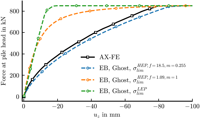
Influence of the axial base relation at fixed initial stiffness and capacity.
The elastic–perfectly plastic relation reaches its cap at approximately \(14\,\mathrm{mm}\) and overpredicts the continuum base resistance by about a factor of three at \(w=0.025D\). A capped Kondner hyperbola (\(m=1\)) also mobilises resistance too rapidly. The exponent \(m=0.255\) provides the gradual intermediate mobilisation required by the continuum curve. The comparison demonstrates representational capability; it does not provide a universal calibration for \(f\) and \(m\).
Base rules with NB=1, 5, 9 and 17 give practically identical global load–settlement curves. NB=9 is retained because its centre-plus-ring geometry transfers moments and preserves the disk moments when all points are active.
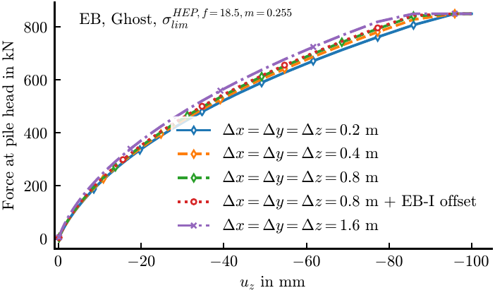
Influence of host discretisation on the base-only response.
Refinement produces a monotonic softening of the pre-cap response; the terminal load is fixed by \(\sigma_{\lim}\pi R^2\). The coarsest and finest meshes differ by approximately \(10\%\) in the intermediate settlement range. The test therefore separates convergence of the mobilisation curve from enforcement of the prescribed capacity.
Extending the elastic ghost zone by a toe half-sphere has negligible influence on the terminal resistance in this benchmark. The conclusion is limited to global axial response with a distributed and explicitly capped base traction; it does not establish equivalence of the local stress field below the toe.
Reproduction with the provided input file (A2): the base resistance follows the capped hyperbola and reaches \(\Delta Q=811\,\mathrm{kN}\) at \(w/D=0.10\) (\(w=80\,\mathrm{mm}\)) and the capacity \(\sigma_{\lim}\pi R^2=850\,\mathrm{kN}\) at \(w=96\,\mathrm{mm}\); the 44 increments require 90 equilibrium iterations in total.
A3: combined shaft and base resistance
The Mohr–Coulomb shaft from A1 and the capped hyperbolic base from A2 are activated together without recalibration. Gaussian soil-stress recovery supplies the shaft-capacity pressure.
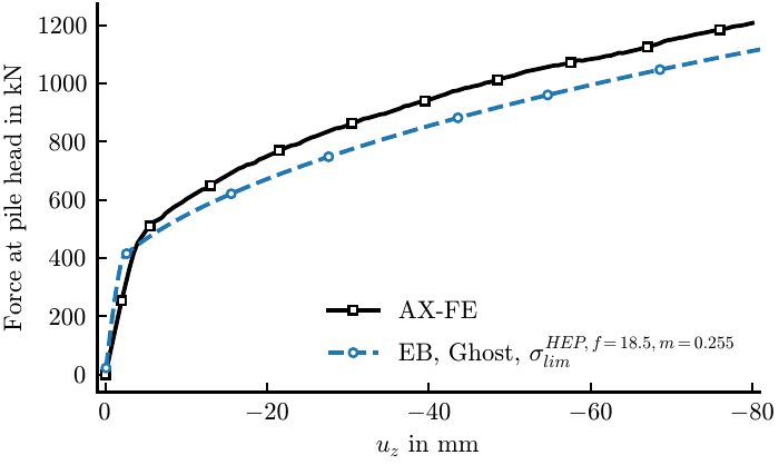
Combined shaft–base response compared with the axisymmetric continuum reference.
The embedded model reproduces the shape of the continuum response over the complete settlement range and remains approximately \(8\%\) below the reference at \(w/D=0.10\). Because neither component is recalibrated, this benchmark checks whether the independently assessed shaft and base relations remain compatible when they act simultaneously.
Reproduction with the provided input file (A3, nb=1, ghost=shaft): \(\Delta Q=1111\,\mathrm{kN}\) at \(w/D=0.10\) (shaft 392 kN, base 705 kN, read from embedded-surface-interactions.res) and \(1212\,\mathrm{kN}\) at \(w=100\,\mathrm{mm}\); the shaft resistance is mobilised within the first 2 mm (\(\Delta Q=387\,\mathrm{kN}\) at \(w=2\,\mathrm{mm}\)), the base resistance follows the capped hyperbola. The 44 increments require 89 equilibrium iterations.
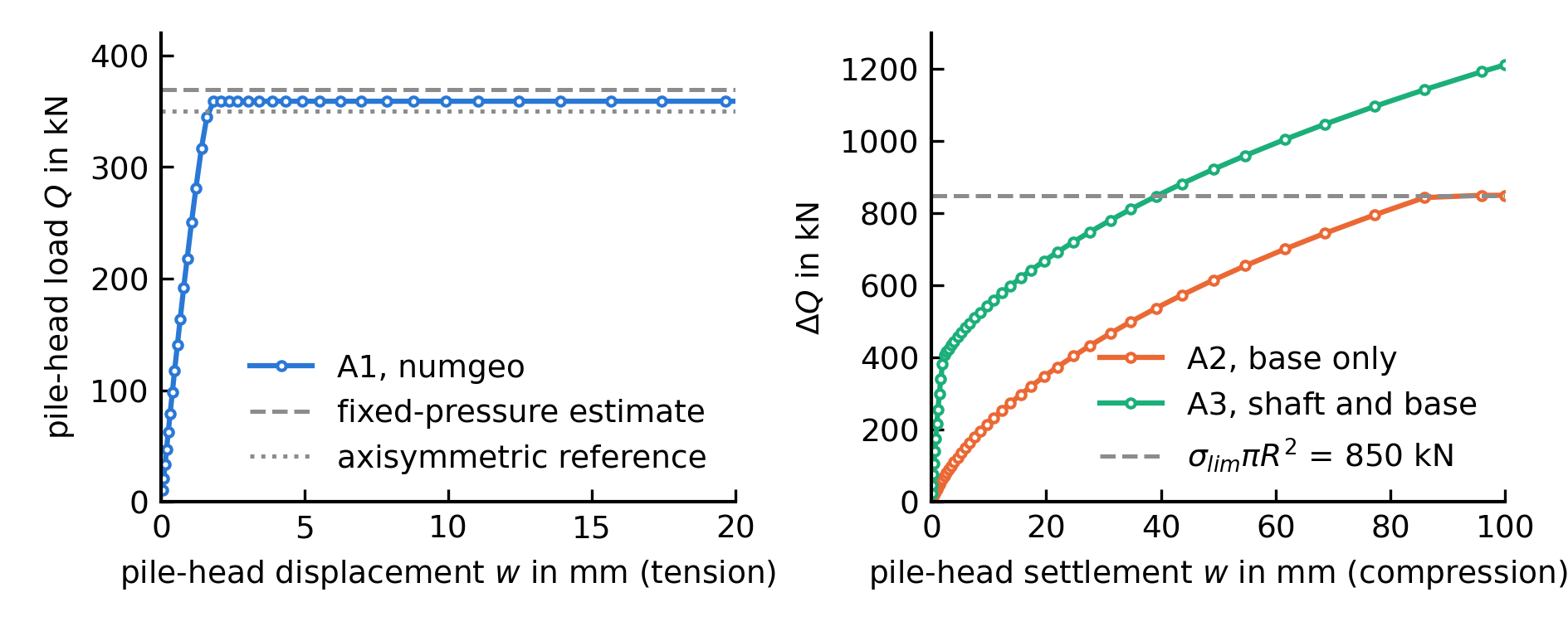
Load-displacement curves obtained with the provided input files: A1 (tension, left; dashed: fixed-pressure estimate 369.3 kN, dotted: axisymmetric reference 350.3 kN) and A2, A3 (compression, right).
Verified implementation components
Together, A1–A3 exercise:
- interface- and soil-stress capacity sources;
- inverse-distance and Gaussian stress recovery;
- one-increment-lagged pressure states;
- shaft return mapping and pressure limiting;
- base envelope, cap and loading history;
- base-disk area and moment integration;
- flat and hemispherical ghost-zone options;
- mesh-size, topology and mesh-position effects;
- simultaneous shaft and base transfer.
-
Andreas-Nizar Granitzer, Franz Tschuchnigg, Haris Felic, Paul Bonnier, and Sandro Brasile. Implementation and appraisal of stress recovery techniques for embedded finite elements with frictional contact. Computers and Geotechnics, 172:106457, 2024. doi:10.1016/j.compgeo.2024.106457. ↩