Pull-out of a grouted anchor (embedded beam, line coupling)
The complete input files of this tutorial (mesh, calculation file, mesh generator and evaluation script) can be downloaded here.
This tutorial shows how to embed a line element - here the grout body of a grouted anchor - into a continuum mesh using *Embedded region, interaction. The grout body is idealised as a truss whose nodes do not need to coincide with the nodes of the soil mesh; the interaction with the surrounding soil is described by distributed interface springs with a stress-dependent (Mohr-Coulomb) skin friction. You will learn
- how to set up a non-conforming guest/host mesh,
- how to install the anchor wished in place after the geostatic step using a material change,
- how to define the interface parameters of the embedded beam, and
- how to evaluate the pull-out resistance against a closed-form estimate.
The corresponding theory is described in the Theory Manual; verification examples with rigid hosts are given in the Benchmark Manual.
Model
We consider a vertical grouted anchor in a 12 m wide and 8 m deep soil block under plane-strain conditions (Figure 1). The grout body has a length of \(L=4.5\) m and a diameter of \(D=0.15\) m; the anchors are installed with an out-of-plane spacing of \(s=2\) m. A tendon connects the grout body to the ground surface, where the anchor is pulled by a prescribed displacement.
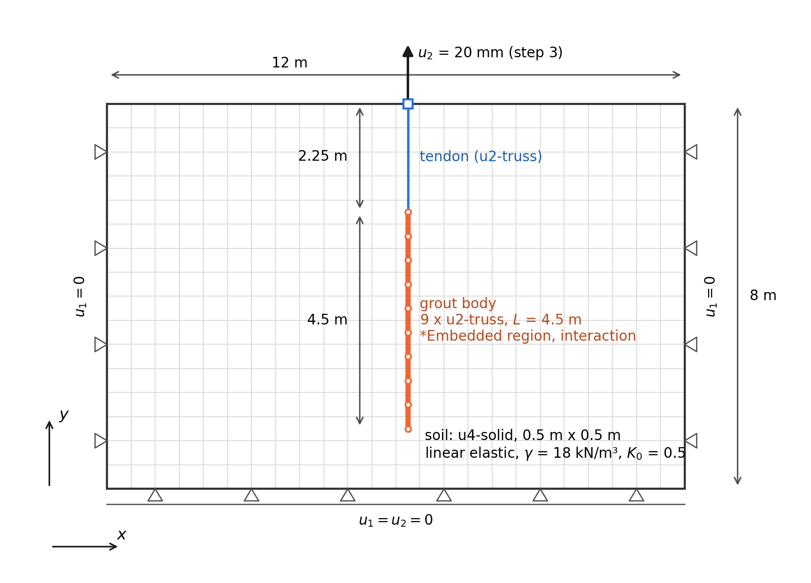
Figure 1. Model of the anchor pull-out test.
The soil is discretised with 384 u4-solid elements of 0.5 m x 0.5 m. The grout body consists of nine u2-truss elements (ten nodes) placed at \(x=6.25\) m, i.e. along the centres of a column of soil elements: the anchor nodes lie at the centroids of the host elements and coincide with no soil node. The tendon is a single u2-truss element from the upper grout node to the ground surface. The mesh file anchor-mesh.inp was generated with the small Python script make_mesh.py contained in the download; it defines the node sets soil, left, right, bottom, grout-nodes and anchor-head and the element sets soil, grout, tendon and anchor. The mesh is included in the calculation file with
*Include, input=anchor-mesh
Materials
The soil is modelled as linear elastic with \(E=30\) MPa, \(\nu=0.3\) and a density of 1.8 t/m³ (\(\gamma=18\) kN/m³ with \(g=10\) m/s²):
*Material, name=sand, phases=1
*Mechanical=linear_elasticity
30000, 0.3
*Density
1.8
The grout body (\(A=\pi D^2/4=0.017671\) m², \(E=20\) GPa) and the tendon (steel strand, \(A=3\) cm², \(E=200\) GPa) are truss elements and require *Truss properties. Two materials are defined for the grout body: a dummy material with negligible stiffness, which is assigned before the installation, and the real grout material:
*Material, name=grout-dummy, phases=1
*Truss properties
0.017671, 1.0
*Density
0.0

*Material, name=grout-material, phases=1
*Truss properties
0.017671, 2.0e7
*Density
0.0

*Material, name=tendon-material, phases=1
*Truss properties
3.0e-4, 2.0e8
*Density
0.0
The materials are assigned to the element sets; the grout body initially receives the dummy material:
*Solid section, elset=soil, material=sand
*Solid section, elset=grout, material=grout-dummy
*Solid section, elset=tendon, material=tendon-material
Why a dummy material?
The embedded interface transmits only the relative displacement between the guest element and the surrounding soil. An anchor that is present from the beginning of the analysis with its real stiffness would participate in the geostatic equilibrium and could attract forces from any settlement of the soil. With the soft dummy material the grout body simply follows the soil during the geostatic step, free of interface forces, and is "installed" afterwards by switching to the real material (Step 2). This is the recommended wished-in-place sequence for anchors, nails and piles.
Initial conditions
The initial stress field is geostatic with \(\sigma_v=-\gamma\,|y|\) and a lateral earth pressure coefficient \(K_0=0.5\) (ground surface at \(y=0\), bottom of the model at \(y=-8\) m):
*Initial conditions, type=stress, geostatic
soil, 0.0, 0.0, -8.0, -144.0, 0.5, 0.5
Embedded region
The grout body is embedded into the soil with the keyword *Embedded region, interaction. We use the Mohr-Coulomb interface law, for which the data line contains the guest and host element sets, the axial and lateral interface stiffnesses \(k_t\) and \(k_n\) (per unit anchor length), the interface cohesion \(c\), the interface friction angle \(\varphi\) and the shear surface per unit anchor length \(A_s\):
*Embedded region, interaction, type=Mohr-Coulomb
grout, soil, 2.0e4, 2.0e4, 20.0, 30.0, 0.2356
- \(k_t=k_n=2\times10^4\) kN/m/m. A mesh-related estimate for the axial stiffness of an anchor row is \(k_t\approx\dfrac{G}{R\ln(1+h/R)}\dfrac{\pi D}{s}\) with the shear modulus of the soil \(G\), the grout radius \(R\) and the element size \(h\), which gives about \(1.8\times10^4\) kN/m/m here. The interface stiffnesses mainly control the displacement at which the skin friction is mobilised; the capacity is governed by \(c\), \(\varphi\) and the stress state.
- \(c=20\) kPa and \(\varphi=30^\circ\) define the skin friction \(\tau_{\mathrm{cap}}=c-\sigma_n\tan\varphi\) with the mean lateral stress \(\sigma_n=\tfrac12(\sigma_{xx}+\sigma_{zz})\) of the soil (compression negative, i.e. compression increases the capacity).
- \(A_s=\pi D/s=\pi\cdot0.15/2.0=0.2356\) m converts the skin friction into a force per unit anchor length of the plane-strain model (one anchor per 2 m).
During the analysis, the capacity of each interface integration point is updated from the converged soil stresses of the previous increment (see the Theory Manual).
Log file
After building the model, numgeo reports in the .log file how many guest elements were embedded, e.g. *Embedded region, interaction: 9 of 9 guest elements of set "GROUT" embedded in host region "SOIL". Guest elements with a node outside the host region are skipped; check this line if an anchor appears to be inactive.
Step 1: geostatic equilibrium
The first step establishes equilibrium between the initial stresses and the self-weight of the soil. The vertical boundaries are supported in horizontal direction and the bottom in both directions; the horizontal displacement of the anchor head (which lies outside the soil and is connected to the model only by the tendon) is fixed to suppress a rigid-body rotation of the tendon:
*Step, name=geostatic, inc=1
*Geostatic
*Body force, instant
soil, grav, 10.0, 0.0, -1.0, 0.0
*Boundary
left, u1, 0.0
right, u1, 0.0
bottom, u1, 0.0
bottom, u2, 0.0
anchor-head, u1, 0.0
*Output, field, vtk, binary
*Node output, nset=soil
u, s
*Node output, nset=grout-nodes
u, s
*End step
Since the prescribed initial stress is in equilibrium with the self-weight, the displacements after this step are zero and the grout body - with its dummy material - is stress free.
Step 2: installation of the anchor
The anchor is installed by assigning the real grout material to the element set grout with *Model change, material. No load is changed in this step; the boundary conditions and body forces are repeated:
*Step, name=installation, inc=1
*Static
1.0, 1.0, 1.0, 1.0
*Model change, material
grout, grout-material
*Body force, instant
soil, grav, 10.0, 0.0, -1.0, 0.0
*Boundary
left, u1, 0.0
right, u1, 0.0
bottom, u1, 0.0
bottom, u2, 0.0
anchor-head, u1, 0.0
*Output, field, vtk, binary
*Node output, nset=soil
u, s
*Node output, nset=grout-nodes
u, s
*End step
Step 3: pull-out test
In the third step the anchor head is pulled upwards by 20 mm in 40 increments. The reaction force at the anchor head is written to the print output together with the displacements of the grout nodes:
*Step, name=pull-out, inc=1000
*Static
0.025, 1.0, 0.001, 0.025
*Body force, instant
soil, grav, 10.0, 0.0, -1.0, 0.0
*Boundary
left, u1, 0.0
right, u1, 0.0
bottom, u1, 0.0
bottom, u2, 0.0
anchor-head, u1, 0.0
*Boundary, amplitude=ramp
anchor-head, u2, 0.02
*Output, field, vtk, binary
*Node output, nset=soil
u, s
*Node output, nset=grout-nodes
u, s
*Output, print
*Node output, nset=anchor-head
u, rf
*Node output, nset=grout-nodes
u
*End step
The amplitude ramp increases the prescribed displacement linearly over the step time:
*Amplitude, name=ramp, type=ramp
0.0, 0.0, 1.0, 1.0
Run the simulation with numgeo inp=anchor-pull-out out=anchor (see Running numgeo). The three steps take a few seconds.
Results
The pull-out force is the vertical reaction force RF2 of the anchor head, available in anchor-print-out/ANCHOR-HEAD_node_436.dat. Figure 2 shows the force versus the head displacement. The response is linear until the skin friction is fully mobilised along the whole grout body at a head displacement of about 3.5 mm; afterwards the anchor slides at a constant force of \(F=45.5\) kN.
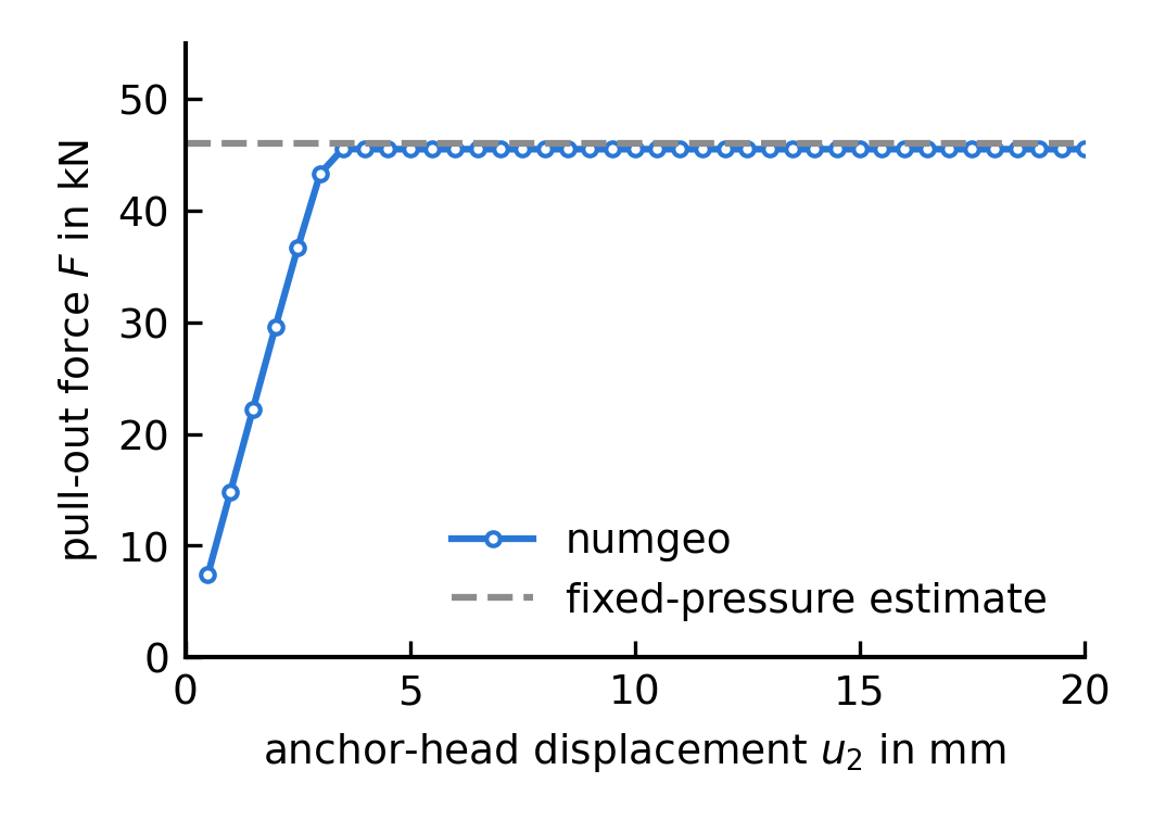
Figure 2. Pull-out force versus anchor-head displacement.
For a check of the result we estimate the capacity by integrating the skin friction over the grout body with the geostatic stresses kept fixed. With \(\sigma_n=K_0\sigma_v=-K_0\gamma z\) (\(z\): depth), the capacity per unit anchor length is \(t_{\mathrm{cap}}(z)=A_s\left(c+\tan\varphi\,K_0\gamma z\right)\), and its integral between the first and the last grout node (\(z_1=2.25\) m, \(z_2=6.75\) m) reads
The simulated capacity of 45.5 kN is 1 % lower: pulling the anchor drags the surrounding (elastic) soil upwards, which slightly reduces the vertical and therefore also the lateral stress around the grout body. Since the interface capacity is evaluated from the current soil stresses, this stress relief reduces the available skin friction - an effect that a fixed-pressure estimate cannot represent.
What to look at in ParaView
Open anchor-all-results.pvd. The grout nodes are contained in the 1D dataset; display the vertical displacement U_2 of the soil and of the anchor with the same colour scale to see the relative displacement (slip) between the two. The soil around the grout body is dragged upwards while the anchor slides.
Python script for plotting the results
import math
import numpy as np
import matplotlib.pyplot as plt

# closed-form estimate (geostatic stresses kept fixed)
gamma, K0 = 18.0, 0.5
c, phi, A_s = 20.0, 30.0, 0.2356
z1, z2 = 2.25, 6.75
L = z2 - z1
F_fp = A_s*(c*L + math.tan(math.radians(phi))*K0*gamma*(z2**2 - z1**2)/2.0)

head = np.genfromtxt('./anchor-print-out/ANCHOR-HEAD_node_436.dat', skip_header=1)
u2, rf2 = head[:, 2], -head[:, 5]

plt.figure(figsize=(9/2.54, 6.5/2.54))
plt.plot(u2*1e3, rf2, '-o', ms=3, mfc='white', label='numgeo')
plt.axhline(F_fp, color='0.55', ls='--', label='fixed-pressure estimate')
plt.xlabel('anchor-head displacement $u_2$ in mm')
plt.ylabel('pull-out force $F$ in kN')
plt.legend(frameon=False)
plt.tight_layout()
plt.savefig('result-anchor-pull-out.png', dpi=300)
Variations
- Replace
type=Mohr-Coulombby the constant-capacity law:*Embedded region, interactionwith the data linegrout, soil, 2.0e4, 2.0e4, 10.0limits the skin friction to \(t_{\mathrm{ult}}=10\) kN/m independent of the stress state (pull-out capacity \(t_{\mathrm{ult}}L=45\) kN). - Refine the soil mesh: the host stress assigned to a guest node is the mean stress of its host element, hence the anchor "sees" the stress gradient with the resolution of the host mesh.
- Use a Mohr-Coulomb soil (
*Mechanical=mohr-coulomb-2) to study the interaction between plastic yielding of the soil and the stress-dependent interface capacity.