Axially loaded pile (embedded beam with interaction surface)
The complete input files of this tutorial (mesh, calculation file, mesh generator and evaluation script) can be downloaded here.
This tutorial shows how to model a single pile with *Embedded region, interaction-surface: the pile is represented by beam elements that are placed into the soil mesh without matching nodes, and the interaction with the soil is described on an implicit cylindrical surface of the pile diameter with a Mohr-Coulomb shaft friction, a nonlinear base resistance and a unilateral (compression-only) contact. Compared with the line coupling of the anchor tutorial, the interaction surface accounts for the pile diameter, the base resistance and the separation between pile and soil, and transfers bending moments through the lever arm of the cross-section. You will learn
- how to prepare a host mesh for an embedded pile,
- how to choose the options and parameters of the interaction surface,
- how to install the pile wished in place after the geostatic step, and
- how to evaluate the load-settlement curve, the shaft and base resistance and the interaction-surface output in ParaView.
The theory is described in the Theory Manual; the benchmarks A0-A3 verify the implementation against closed-form and continuum solutions.
Model
A bored pile with a diameter of \(D=0.6\) m and an embedded length of \(L=8\) m is installed in a homogeneous sand and loaded in compression to a head settlement of \(w=0.1D=60\) mm (Figure 1). The soil block is 8 m x 8 m in plan and 12 m deep; the pile is located at its centre.
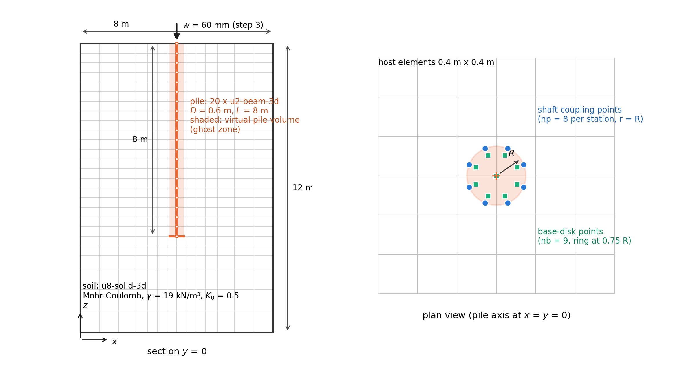
Figure 1. Model of the axially loaded pile: graded host mesh (left) and pile with interaction surface and base disk (right).
Mesh
The soil is discretised with u8-solid-3d elements. The mesh is graded towards the pile: 0.4 m next to the pile axis, growing to 0.8 m at the lateral boundaries, 0.4 m along the pile and coarser below the toe (5096 elements, 6075 nodes). The pile consists of 20 u2-beam-3d elements of 0.4 m between the ground surface (\(z=0\)) and the toe (\(z=-8\) m). The mesh file pile-mesh.inp was generated with the script make_mesh.py contained in the download; it defines the node sets soil, x-min, x-max, y-min, y-max, bottom, pile-nodes, pile-head, pile-toe and the element sets soil and pile.
Two requirements of the interaction surface are worth noting when preparing a mesh:
- The pile nodes must be separate nodes with their own labels. Their coordinates may coincide with soil nodes (as in this example, where the pile axis coincides with a column of soil nodes), but a node shared by a beam and a soil element is rejected.
- The host elements should be smaller than the pile diameter near the pile. The coupling points are generated on the pile circumference (here at \(R=0.3\) m from the axis), hence elements of 0.4 m resolve the interaction surface reasonably. Moreover, the elastic ghost zone (see below) is realised at the integration points of the host elements inside the pile volume; with 8-point hexahedra centred on the pile axis, integration points lie inside the pile only if the element size is smaller than \(1.22D\).
*Include, input=pile-mesh
Materials
The sand is modelled with the Mohr-Coulomb model (\(E=40\) MPa, \(\nu=0.3\), \(c=2\) kPa, \(\varphi=30^\circ\), \(\psi=0\)) and a density of 1.9 t/m³:
*Material, name=sand, phases=1
*Mechanical=mohr-coulomb-2
40000, 0.3, 2.0, 30.0, 0.0, 0.0
*Density
1.9
The pile is a concrete beam with \(E=30\) GPa, \(G=12.5\) GPa, \(A=\pi D^2/4=0.28274\) m², \(I=\pi D^4/64=0.0063617\) m⁴ and \(J=2I\) (*Beam properties). As in the anchor tutorial, a soft dummy material is assigned before the installation so that the pile follows the soil during the geostatic step free of interface forces:
*Material, name=pile-dummy, phases=1
*Beam properties
0.28274, 1.0, 0.4167, 0.0063617, 0.0063617, 0.0127235, 0.9, 0.9
*Density
0.0

*Material, name=pile-concrete, phases=1
*Beam properties
0.28274, 3.0e7, 1.25e7, 0.0063617, 0.0063617, 0.0127235, 0.9, 0.9
*Density
0.0

*Solid section, elset=soil, material=sand
*Solid section, elset=pile, material=pile-dummy
The pile density is set to zero: the soil inside the virtual pile volume is not removed from the mesh, so its weight already acts on the model (mass-neutral convention).
Initial stress
*Initial conditions, type=stress, geostatic
soil, 0.0, 0.0, -12.0, -228.0, 0.5, 0.5
Embedded region
The pile is coupled to the soil with the following keyword line and data line:
*Embedded region, interaction-surface, type=Mohr-Coulomb, sigma=soil, recovery=gaussian, ghost=yes, baselaw=hyperbolic, bfac=18.48, bexp=0.2553
pile, soil, pile-toe, 0.6, 6.0e4, 6.6e5, 4.2e5, 1.0, 22.0, 1500.0, 60000.0, 0.3
The options select the constitutive behaviour of the interaction surface:
type=Mohr-Coulomb- the shaft friction is limited by \(t_{\mathrm{cap}}=c+p\tan\varphi\) with the interface parameters \(c=1\) kPa and \(\varphi=22^\circ\) (data line). Both the axial and the circumferential traction share this capacity (Coulomb circle).sigma=soil, recovery=gaussian- the pressure \(p\) entering the capacity is the compressive normal stress of the soil, recovered at every coupling point from the integration points of the neighbouring host elements with Gaussian weights. With this choice the shaft capacity follows the stress state of the soil and is largely independent of the normal stiffness \(k_n\). The alternativesigma=interfaceuses the pressure of the normal spring itself.tension=no(default) - the contact is unilateral: a shaft point separates from the soil when the total contact pressure (initial pressure plus spring pressure) becomes tensile; it then transfers no tangential traction and releases its initial pressure. The base disk opens when its axial traction becomes tensile. For a pile in compression the shaft remains closed.baselaw=hyperbolic, bfac=18.48, bexp=0.2553- the base resistance is mobilised along a capped generalised hyperbola with the initial stiffness \(k_b\), the capacity \(\sigma_{\lim}=1500\) kPa and the shape parameters \(f=18.48\) and \(m=0.2553\) (values fitted to a continuum reference in benchmark A2). The elastic-perfectly plastic alternative (baselaw=elastic-plastic) mobilises the base much faster.ghost=yes- the soil integration points inside the pile volume and in a half-sphere below the toe respond linear elastically with \(E_{\mathrm{ghost}}=60\) MPa and \(\nu_{\mathrm{ghost}}=0.3\) (last two entries of the data line), so that the soil that "occupies" the pile cannot yield under the coupling forces.np=8andnb=9(defaults) - eight coupling points around the circumference at every beam integration station and a base disk with a centre point and eight ring points.
The data line contains the guest element set, the host element set, the node set of the toe node (pile-toe, an end node of the pile), the diameter \(D\), the stiffnesses \(k_t\), \(k_n\) and \(k_b\) (force per area per length), the interface strength, the base capacity and the ghost parameters. The interface stiffnesses are penalty-like parameters that should scale with the soil stiffness and the host element size \(h\); the estimates of the Theory Manual with \(G=15.4\) MPa, \(R=0.3\) m, \(h=0.4\) m and \(\nu_i=0.45\) give \(k_t\approx6\times10^4\) kN/m³, \(k_n=11k_t\approx6.6\times10^5\) kN/m³ and \(k_b\approx4.2\times10^5\) kN/m³, which are used here. A tenfold change of these values has a small influence on the load-settlement curve; a sensitivity check is nevertheless recommended for every new application.
Log file
After building the model, numgeo reports the number of coupled guest elements and coupling points, the base disk and the number of host integration points switched to the ghost response:
*Embedded region, interaction-surface: 20 of 20 guest elements of set "PILE" coupled to host region "SOIL" (320 coupling points)
   -> base disk generated at 1 toe node(s) (9 base coupling points)
   -> ghost (elastic) zone: 164 host integration points switched to the linear elastic ghost response
A warning is issued if the ghost zone is active but no integration point lies inside the pile volume (host elements too large), if a toe node is not an end node of a coupled beam, or if none of the base points of a toe node lies inside the host region.
Step 1: geostatic equilibrium
*Step, name=geostatic, inc=1
*Geostatic
*Body force, instant
soil, grav, 10.0, 0.0, 0.0, -1.0
*Boundary
x-min, u1, 0.0
x-max, u1, 0.0
y-min, u2, 0.0
y-max, u2, 0.0
bottom, u1, 0.0
bottom, u2, 0.0
bottom, u3, 0.0
*Output, field, vtk, binary
*Node output, nset=soil
u, s, embedded
*End step
The output variable embedded requests the interaction-surface datasets (see Results). During the geostatic step the initial contact pressure of the interaction surface is recovered from the soil stresses; it is frozen at the beginning of the next step.
Step 2: installation of the pile
*Step, name=installation, inc=1
*Static
1.0, 1.0, 1.0, 1.0
*Model change, material
pile, pile-concrete
*Body force, instant
soil, grav, 10.0, 0.0, 0.0, -1.0
*Boundary
x-min, u1, 0.0
x-max, u1, 0.0
y-min, u2, 0.0
y-max, u2, 0.0
bottom, u1, 0.0
bottom, u2, 0.0
bottom, u3, 0.0
*Output, field, vtk, binary
*Node output, nset=soil
u, s, embedded
*End step
Step 3: axial loading
The pile head is pushed down by 60 mm, using the amplitude ramp (linear over the step time) with an initial increment of 1 % of the step and a maximum increment of 5 %:
*Step, name=loading, inc=1000
*Static
0.01, 1.0, 0.001, 0.05
*Body force, instant
soil, grav, 10.0, 0.0, 0.0, -1.0
*Boundary
x-min, u1, 0.0
x-max, u1, 0.0
y-min, u2, 0.0
y-max, u2, 0.0
bottom, u1, 0.0
bottom, u2, 0.0
bottom, u3, 0.0
*Boundary, amplitude=ramp
pile-head, u3, -0.06
*Output, field, vtk, binary
*Frequency=5
*Node output, nset=soil
u, s, embedded
*Output, print
*Node output, nset=pile-head
u, rf
*Node output, nset=pile-toe
u
*End step
Run the simulation with numgeo inp=pile-axial out=pile ncpus=4. The analysis takes a few minutes.
Results
Load-settlement curve
The pile-head load is the vertical reaction force RF3 of the head node (pile-print-out/PILE-HEAD_node_6076.dat). Figure 2 shows the load-settlement curve: the shaft friction is mobilised within the first two millimetres (about 250 kN), whereas the base resistance increases gradually along the hyperbolic mobilisation law and reaches its capacity \(\sigma_{\lim}\pi R^2=424\) kN at a head settlement of about 55 mm. For the chosen shape parameters the cap is reached at \(s^*=\dfrac{f\sigma_{\lim}}{k_b}(f^m-1)^{-1/m}=45\) mm of base penetration. The total resistance at \(w=60\) mm is 664 kN (shaft 240 kN, base 424 kN).
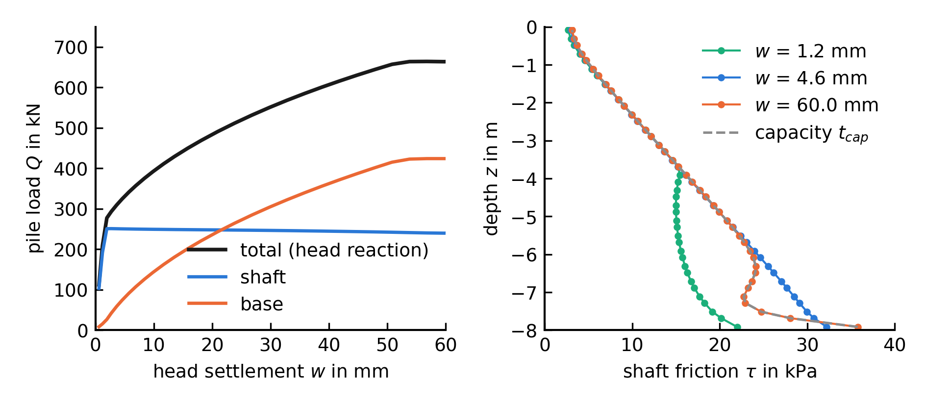
Figure 2. Load-settlement curve of the pile with the contributions of shaft and base (left) and distribution of the shaft friction along the pile at three settlements (right).
Shaft and base resistance
The diagnostic file embedded-surface-interactions.res in the working directory contains, for every converged increment, one line per shaft coupling point (position, tributary area, axial, circumferential and normal traction, capacity, recovered soil stress, slips and pressures) and one line per base point (position, area, traction vector, axial traction, in-plane traction, capacity and history). Summing t_ax * area over the shaft points and over the base points gives the shaft and base resistance shown in Figure 2 (script below); their sum equals the head reaction. The right-hand diagram of Figure 2 shows the shaft friction along the pile: at \(w=1.2\) mm the lower half of the shaft is still elastic, at \(w=4.6\) mm the friction equals the capacity \(t_{\mathrm{cap}}=c+p\tan\varphi\) everywhere. Since the capacity pressure \(p\) is the recovered soil stress, the skin friction increases with depth and changes slightly during loading, when the soil stresses around the toe are altered by the base pressure. Delete the file before re-running the analysis in the same directory: it is opened in append mode.
Visualisation in ParaView
Open pile-all-results.pvd. Because the output variable embedded was requested, the multiblock dataset contains two additional blocks per output increment: the pile (pile-embedded-beam-1-...) and the interaction surface (pile-embedded-surface-1-...). The interaction surface is a reconstruction of the shaft (one planar facet per coupling point) and of the base disk; its cell data include the traction components t_ax, t_cir, t_n, the capacity t_cap, the mobilisation \(\|\mathbf t_t\|/t_{\mathrm{cap}}\), the recovered soil stress Sigma_n and the slip magnitude. Colour the surface by t_ax to see the shaft friction, by Mobilisation to see where the interface slides, and by SurfacePart to distinguish shaft (0) and base (1). The small gaps between the axial bands of the reconstructed surface separate the facets of neighbouring integration stations and have no mechanical meaning.
Python script for plotting the results
import numpy as np
import matplotlib.pyplot as plt

# pile-head load-settlement curve (step 3 starts at t = 2)
head = np.genfromtxt('./pile-print-out/PILE-HEAD_node_6076.dat', skip_header=1)
w, Q = -head[:, 3]*1e3, head[:, 6]

# shaft and base resistance from the diagnostic file
shaft, base, tshaft = [], [], []
with open('./embedded-surface-interactions.res') as f:
    for line in f:
        if line.startswith('** step'):
            shaft.append(0.0); base.append(0.0); tshaft.append([])
        elif line.startswith('**') or not line.strip():
            continue
        else:
            v = [float(x) for x in line.split(',')]
            if len(v) >= 16:                  # shaft point: area = v[5], t_ax = v[6]
                shaft[-1] += v[6]*v[5]
                tshaft[-1].append((v[4], v[6]))
            else:                             # base point: area = v[5], t_ax = v[9]
                base[-1] += v[9]*v[5]
shaft, base = np.array(shaft), np.array(base)
n = len(w)                                    # the last n blocks belong to step 3
shaft, base = shaft[-n:], base[-n:]

fig, ax = plt.subplots(1, 2, figsize=(16/2.54, 6.5/2.54))
ax[0].plot(w, Q, color='0.1', label='total')
ax[0].plot(w, shaft, color='#2a78d6', label='shaft')
ax[0].plot(w, base, color='#eb6834', label='base')
ax[0].set_xlabel('head settlement $w$ in mm')
ax[0].set_ylabel('pile load $Q$ in kN')
ax[0].legend(frameon=False)
for k, col in zip([1, 5, len(w)-1], ['#1baf7a', '#2a78d6', '#eb6834']):
    z, t = np.array(tshaft[len(tshaft)-n+k]).T
    order = np.argsort(z)
    ax[1].plot(t[order], z[order], '.', color=col, label='$w$ = %.1f mm' % w[k])
ax[1].set_xlabel(r'shaft friction $\tau$ in kPa')
ax[1].set_ylabel('depth $z$ in m')
ax[1].legend(frameon=False)
plt.tight_layout()
plt.savefig('result-pile-axial.png', dpi=300)
Variations
- Set
tension=yesto compare with bilateral springs, orghost=noto keep the real soil inside the pile volume, and observe the influence on the load-settlement curve. - Replace
baselaw=hyperbolic, bfac=18.48, bexp=0.2553bybaselaw=elastic-plastic: the base resistance then reaches \(\sigma_{\lim}\pi R^2\) at a settlement of only \(\sigma_{\lim}/k_b\approx3.6\) mm. - Apply a horizontal head displacement instead of the settlement: the trailing side of the shaft separates once the initial contact pressure is released (
t_ax,t_cirandMobilisationvanish there andt_nshows the released pressure \(-p_{\mathrm{ini}}\)), the bending moment is transferred through the lever arm of the interaction surface, and the base disk slides. - Add further piles (each with its own toe node in
pile-toe) to model a pile group with a single*Embedded regiondefinition.